Variability diagnostics
In MCRA, the nominal run might be followed by an uncertainty analysis to assess the uncertainty limits (e.g. 2.5 and 97.5%) of the nominal percentiles (e.g. p50, p95, p99, p99.9, p99.99) of the exposure or risk distribution. For these percentiles, the nominal run of an acute assessment consists of preferably 100.000 iterations, the uncertainty analysis preferably of 100 runs with 10.000 iterations each. Note that for the percentile p99.99 the minimal number of iterations should be 10.000. Likewise, to estimate uncertainty limits of 2.5 and 97.5%, the minimal number of bootstrap runs should be 100.
In general, the number of iterations and bootstrap runs will be restricted due to limited computational resources or simulation runs that are time consuming. MCRA offers a diagnostic tool to visualize whether the estimated percentiles and uncertainty limits are stable or vary due to small simulation runs with limited number of iterations and uncertainty runs.
The diagnostic tool focus on the stability of the percentiles or, re-frasing, quantify 1) the amount of Monte Carlo variability and 2) the amount of variability due to resampling e.g. consumption and monitoring data or others sources of uncertainty. By quantifying both quantities, the influence of both sources of variability on the estimated value of the percentiles is assessed.
The diagnostics are displayed in a number of graphs (as many as the number of specified percentiles). For each percentile, the graph is used to draw inference about the optimal number of MC-iterations, the number of uncertainty runs and the number of iterations in each uncertainty run.
In the section below it is assumed that the nominal run consists of 100.000 iterations and uncertainty (95% confidence) is assessed with 100 uncertainty runs of 10.000 iterations each.
To make inference, the set of nominal (Monte Carlo) values is split in 2 samples of 50.000 iterations each, 4 samples of 25.000 each, 8 samples of 12.500 each etc. By doing so, we get \(n\) partitions of samples and in each partition we have \(2^n\) samples of size 100.000/\(2^n\). In each partion, the percentiles of the available samples are estimated and the standard deviation of the percentiles. So in partition \(n\) = 1, the estimate of the standard deviation is based on 2 percentiles derived from samples of size 50.000; in partition \(n\) = 2, the estimate of the standard deviation is based on 4 percentiles derived from samples of size 25.000, etc. The estimated standard deviations are plotted against the number of MC-iterations per sample of each partition. It is expected that the standard deviation decreases as a function of sample size, so for larger sample sizes MC-variability decreases. For each standard deviation the 90% confidence limits are calculated.
A similar procedure is applied to the 100 uncertainty runs (of size 10.000). In each uncertainty run the percentiles are estimated. Then, in partition \(n\) = 1, percentiles are estimated on the first 10.000/2 = 5000 iterations of each sample; in partition \(n\) = 2 percentiles are estimated on the first 10.000/4 = 2500 iterations of each sample, etc. Then standard deviations of the percentiles of the partitions of 100 x 10.000, 100 x 5000, 100 x 2500, etc are estimated and plotted against the number of iterations in each partition. It is expected that the standard deviation decreases as a function of sample size.
In Figure 12, the estimates and uncertainty limits are displayed. In Figure 11, the diagnostics are dlotted
Red dots: standard deviation (sd) of percentile estimates between subsets of simulations. Error bars indicate parametric 90% confidence interval for the sd.
Blue dots: standard deviation of percentile estimates between uncertainty iterations of subsets of simulations. The red square indicates the specified number of iterations (10000) of an uncertainty run.
Each blue dot represents the standard deviation of 100 percentiles
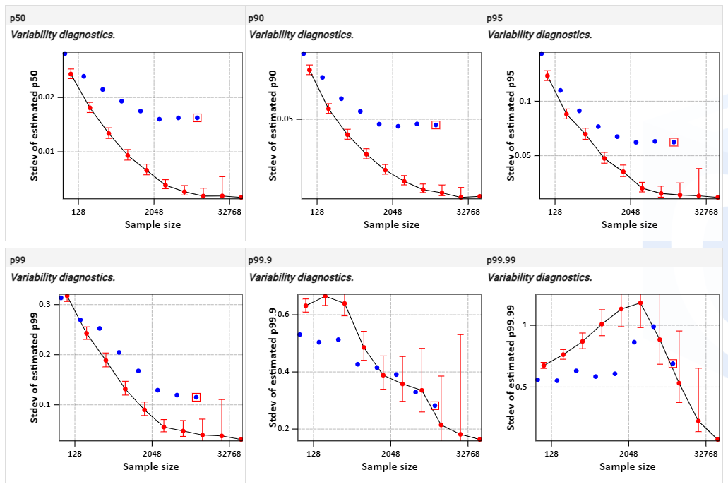
Figure 11 Variability diagnostics for percentiles p50, p90, p95, p99, p99.9 and p99.99.
For percentages, p50, p90, p95 and p99 the curves of the nominal estimates are smooth. For the extreme percentiles, p99.9 and p99.99, patterns do not monotonically decrease and vary, indicating that percentile estimates are variable. Also the 90% confidence interval around the sd’s are much larger than for the smaller percentiles. An general conclusion is that percentiles and uncertainty limits for p50, p99, p95 and p99 are stable. The percentile of the p99.99 is unstable meaning that running the simulation with a different initialisation seed estimates will vary. The percentile p99.9 is an intermediate case.
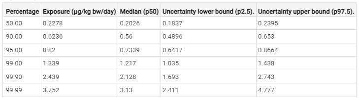
Figure 12 Exposure estimates for percentiles p50, p90, p95, p99, p99.9 and p99.99 with 95% confidence limits

Figure 13 Boxplots for summary statistics for percentiles p50, p90, p95, p99, p99.9 and p99.99 with 95% confidence limits
The boxplots for uncertainty show the p25 and p75 as edges of the box, and p2.5 and p97.5 as edges of the whiskers. The reference value is indicated with the dashed black line, the median with the solid black line within the box. Outliers are displayed as dots outside the wiskers.