Sparse nonnegative matrix underapproximation
Starting point to identify major mixtures of substances using exposure data was to use Non-negative Matrix Factorization (NMF). Non-negative Matrix Factorization was proposed by Lee and Seung (1999) and Saul and Lee (2002) and deals specifically with non-negative data that have excess zeros such as exposure data. Zetlaoui et al. (2011), introduced this method in food risk assessment to define diet clusters.
The NMF method was then implemented by Béchaux et al. (2013) in order to identify food consumption patterns and main mixtures of pesticides to which the French population was exposed using TDS exposure to 26 priority pesticides.
At the start of the Euromix project ideas had evolved: to obtain less components per mixture experiments were made using Sparse Nonnegative Matrix Factorization (SNMF) (Hoyer (2004)). This method was found not to give stable solutions. Better results were obtained with Sparse Nonnegative Matrix Underapproximation (SNMU) (Gillis and Plemmons (2013)). This model also fits better to the problem situation because also the residual matrix after extracting some mixtures should be nonnegative. The SNMU method has been implemented in MCRA.
Indeed, NMF may be used to identify patterns or associations between substances in exposure data. NMF can be described as a method that finds a description of the data in a lower dimension. There are standard techniques available such as principal components analysis or factor analysis that do the same, but their lower rank representation is less suited because they contain negative values which makes interpretation hard and because of the modelling with a Gaussian random vectors which do not correctly deal with the excess of 0 and non-negative data. The NMF solution approximates a non-negative input matrix (i.c. exposure data) by two constrained non-negative matrices in a lower dimension such that the product of the two is as close as possible to the original input matrix. In Figure 60, the exposure matrix \(M\) with dimensions \(m\) (number of substances) and \(n\) (number of intake days or persons) is approximated by matrix \(U\) and \(V\) with dimensions \((m \times k)\) and \((k \times n)\) respectively, where \(k\) represents the number of mixtures. Matrix \(U\) contains weights of the substances per mixture, matrix \(V\) contains the coefficients of presence of mixtures in exposure per intake day or person. \(M\) is non-negative (zero or positive) and \(U\) and \(V\) are constraint to be non-negative. The minimization criterion is: \(||M – UV||2\) such that \(U \geq 0\) and \(V \geq 0\).
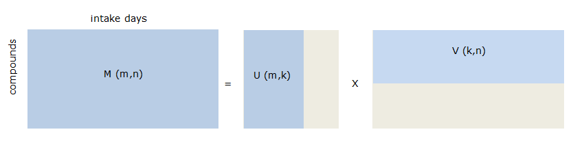
Figure 60 NMF approximation of exposure data
The solution found by NMF contains zeros, but mixtures still contain many components which complicates interpretability. Therefore, the Sparse Nonnegative Matrix Underapproximation (SNMU) (Gillis and Plemmons (2013)) which also provide sparse results was investigated. The SNMU has also some nice features well adapted to the objective of the Euromix project: the solution is independent of the initialization and the algorithm is recursive. Consequently, the SNMU method which is based on the same decomposition process as the NMF was the one implemented in MCRA.
SNMU is initialized using an optimal nonnegative rank-one approximation using the power method (https://en.wikipedia.org/wiki/Power_iteration). This initialization is based on a singular value decomposition and results in general in a unique solution that is sparse. The SNMU algorithm is called recursive because after identifying the first optimal rank-one underapproximation \(u_{1}v_{1}\), the next rank-one factor is recovered by subtracting \(u_{1}v_{1}\) from \(M\) and applying the same factorization algorithm to the remainder \(M - u_{1}v_{1}\). The solution \(u_{1}v_{1}\) is called a rank-one underapproximation because an upper bound constraint is added to ensure that the remainder \(M - u_{1}v_{1}\) is non-negative. For Matlab code see: https://sites.google.com/site/nicolasgillis/code.
For each mixture, a percentage of explained variance is calculated. \(M\) is the exposure matrix with \(m\) rows (substances) and \(n\) columns (individuals or individual days) \(S_{t}\) is sum of squared elements of \(M\):
Apply SNMU on \(M\), then for the first mixture:
\(u\) is \(m \times 1\) vector, contains weights of the mixture.
\(v\) is \(1 \times n\) vector, contains presence of mixture in exposure per individual.
Calculate residual matrix \(R\):
\(R = M - uv\)
Calculate \(S_{r}\), residual sum of squared elements of R:
Percentage explained variance first mixture \((k = 1)\) is:
For the second mixture:
continue with residual matrix \(R\) (replace \(M\) by \(R\)),
estimate \(u\) and \(v\),
calculate new residual matrix \(R\)
calculate \(S_{r}\), residual sum of squared elements of \(R\)
Percentage explained variance second mixture \((k=2)\) is:
The last term is de percentage explained variance of the first mixture. Continue with the third mixture etc….
Exposure matrix
Basically, exposure is calculated as consumption x concentration. By summing the exposures from the different foods for each substance per person day separately, the exposure matrix for mixture selection is estimated:
where \(y_{ijc}\) is the exposure to substance \(c\) by individual \(i\) on day \(j\) (in microgram substance per kg body weight), \(x_{ijk}\) is the consumption by individual \(i\) on day \(j\) of food \(k\) (in g), \(c_{ijkc}\) is the concentration of substance \(c\) in food \(k\) eaten by individual \(i\) on day \(j\) (in mg/kg), and \(\mathit{bw}_{i}\) is the body weight of individual \(i\) (in kg). Finally, \(p\) is the number of foods accounted for in the model. More precisely, for an acute or short term risk assessment, the exposure matrix summarises the \(y_{ijc}\) with columns denoting the individual-days \((ij)\) and rows denoting the substances \((c)\). Each cell represents the sum of the exposures for a substance on that particular day. For a chronic or long term risk assessment, the exposure matrix is constructed as the sum of all exposures for a particular substance averaged over the total number of intake days of an individual (substances x persons). So each row represents a substance and a column an individual. Each cell represents the observed individual mean exposure for a substance for that individual. Note that in the exposure calculation, the concentration is the average of all residue values of a substance.
When relative potency factors (RPF) are available then exposures are multiplied by the RPF and thus exposures to the different substances are on the same and comparable scale (toxicological scale). In this case, the selection of the mixture is risk-based. In some cases, RPFs may not be available. In this case exposure to different substances, even in the same unit, may lead to very different effect. To give all substances an equal weight a priori and avoid scaling effect, a standardisation of the data can be applied as done in Béchaux et al. (2013). In this case, all substances are assigned equal mean and variance, and the selection of the mixtures will work on patterns of correlation only. Then mixture selection is not risk-based anymore but, what could be called, co-exposure-based.
Finally, in the mixture selection module of MCRA, the SNMU expects RPF data for a risk-based selection. If not available, the user should provide alternative RPF data, e.g. values 1 for a purely exposure-based selection, or lower-tier estimates (e.g. a maximum value on RPF thought possible).
Mechanisms to influence sparsity
Two mechanisms to influence sparsity are available. The SNMU algorithm incorporates a sparsity parameter and by increasing the value, the final mixtures will be more sparse (sparsity close to 0: not sparse; sparsity close to 1: sparse). The other approach is by using a subset of the exposure matrix based on a cut-off value for the MCR. High ratios correspond to high co-exposure, so it is reasonable to focus on these (person) days and not include days where exposure is received from a single substance (ratio close to 1). To illustrate the combined use of MCR and the sparsity parameter, the French steatosis data (39 substances, 4079 persons) are used and person days with a ratio > 5 (see Figure 55) are selected yielding a subset of 139 records.
In Figure 61, the effect of using a cut-off level is immediately clear. The number of substances of the first mixture is 17 whereas in the unselected case only 4 substances were found The three plots show the influence of increasing the sparsity parameter from 0 to 1 on the number of substances in the mixture. For values close to 0, the mixture contains 17 substances. For values > 0.4 the number of substances in the mixture drops to 3.
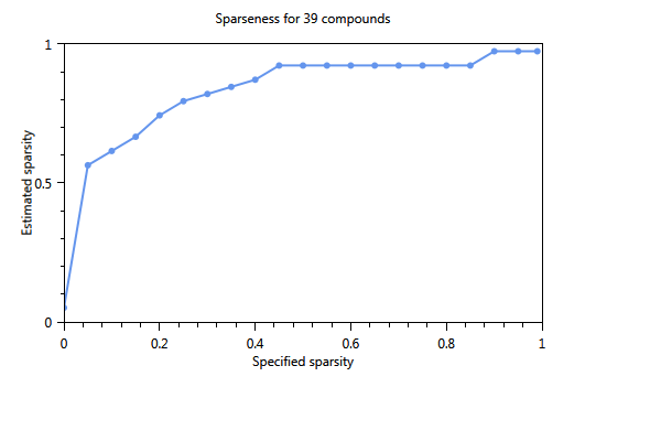
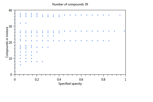
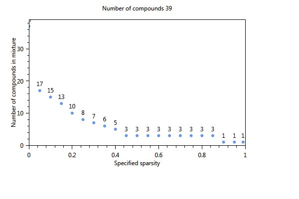
Figure 61 Influence of the specified sparsity parameter on the realized sparsity, n = 139
In Figure 62 and Figure 63 the sparsity parameter is set to 0.0001 (not sparse) and 0.4 (sparse), respectively. This leads to mixtures containing different number of substances.

Figure 62 Heatmap for a solutions with 10 mixtures. The sparsity is set to 0 (not sparse). Each mixture contains many substances (see also Figure 63).

Figure 63 Heatmap for a solutions with 10 mixtures. The sparsity is set to 0.4 (sparse). Mixtures contain less substances compared to Figure 62.
As mentioned before, one of the nice features of the SNMU algorithm is its recursive character which results in identical mixtures. In Figure 64 and Figure 65, two U matrices are visualized. In the upper plot 4 mixtures are estimated, in the lower plot the solution for 5 mixtures is shown. Because of the ordering the plots look different, but a closer inspection of the first 4 mixtures of each solution shows that they are the same. In both figures, mixture 1 contains Imazalil, Thiacloprid, Deltamethrin (cis-deltamethrin) and Deltamethrin including other mixture.

Figure 64 Heatmap for solution with 4 mixtures. The first 4 mixtures in Figure 64 and Figure 65 are identical.

Figure 65 Heatmap for solution with 5 mixtures. The first 4 mixtures in Figure 64 and Figure 65 are identical.