Model-Then-Add

The traditional approach can be termed the Add-Then-Model approach, because adding over foods precedes the statistical modelling of usual exposure. MCRA offers, as an advanced option, an alternative approach termed Model-Then-Add (van der Voet et al. 2014). In this approach the statistical model is applied to subsets of the diet (single foods or food groups), and then the resulting usual exposure distributions are added to obtain an overall usual exposure distribution. The advantage of such an approach is that separate foods or food groups may show a better fit to the normal distribution model as assumed in all common models for usual exposure (including MCRA’s betabinomial-normal (BBN) model and logisticnormal-normal model (LNN)). That this principle can work in practice was shown in previous work (de Boer et al. 2009 [de Boer et al., 2009], Slob et al. 2010 [Slob et al., 2010], Goedhart et al. 2012) [Goedhart et al., 2012], and a simulation model was developed and implemented in MCRA 7.1 to show how multimodal distributions can arise from adding unimodal distributions of foods that are not always consumed (Slob et al. 2010 [Slob et al., 2010], de Boer and van der Voet 2011, [de Boer et al., 2011]). For specific cases involving separate modelling of dietary supplements and the rest of the diet, proposals have been made (Verkaik-Kloosterman et al. 2011) [Verkaik-Kloosterman et al., 2011]. However, a practical approach to apply the Model-Then-Add approach to general cases of usual exposure estimation was still missing. Therefore a module in MCRA was developed to implement such an approach based on a visual inspection of a preliminary estimate of the usual exposure distribution using the Observed Individual Means (OIM) method.

The Model step

At this stage of development the division of foods into a number of food groups is performed in an interactive process, where the MCRA user is presented with a visual display (see example in Figure 28) which shows:

1. The OIM distribution represented as a histogram, where each bar shows the frequency of exposures (summed over foods) of individuals in a certain exposure interval; each bar is subdivided according to the contributions of the individual foods contributing to those exposures (left panel Figure 28).

2. The contributions graph, where each of the bars in the OIM histogram is expanded to 100%. This graph allows a better view of the lower bars in the OIM histogram.

The visual display identifies the nine foods that contribute most to the total exposure; the remaining foods are grouped in a rest category to avoid identification problems because of too many colours (right panel Figure 28).

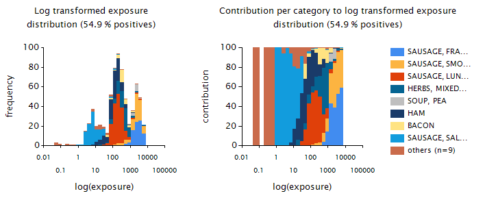
Figure 28 Left panel: OIM usual exposure distribution to smoke flavours via the different foods (excluding the zero exposures) in young children; right panel: Contribution of foods to exposures within each bar of the OIM distribution histogram.

The user has now the possibility to select one or more foods and to split these from the main exposure histogram. A separate graph shows the OIM distribution for the split-off food or food group. The graphs for the main group (now called the rest group) are adapted to show the OIM distribution and the contributions for the remaining foods only (see Figure 29 upper two panels). This splitting-off can be repeated several times for other foods or food groups. In this way the user can try to obtain foods or food groups that show unimodal OIM distributions. If the result is not what is intended, a food or food group can be added again to the rest group. Per split-off food or food group the usual exposure can be modelled using either BBN or LNN, with a logarithmic or power transformation. The rest group will always be modelled as OIM. It is possible that the rest group is empty, when the total exposure via the different split-off foods and /or food groups is modelled with BBN or LNN.

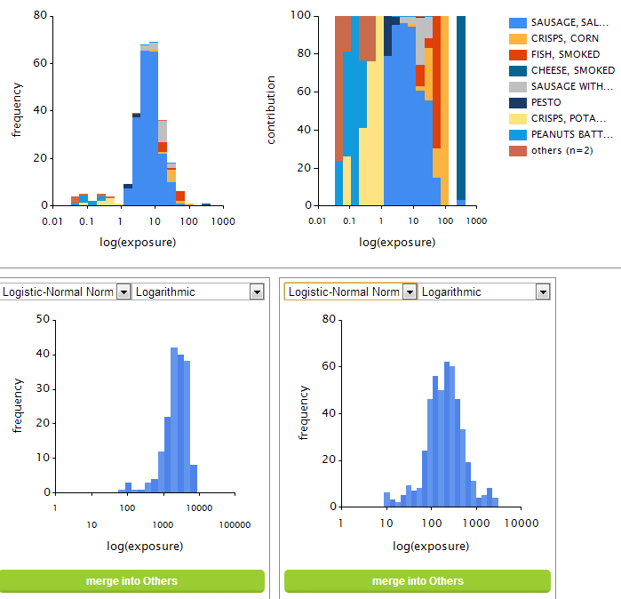
Figure 29 Result of a selection into two split-off groups and a rest group. The graph bottom left represents the exposure via a food group containing ‘Sausage, frankfurter’ and ‘Sausage, smoked cooked’. The graph bottom right represents the exposure via a food group containing ‘Sausage, luncheon meat’, Herbs, mixed, main brands, not prepared’, ‘Soup, pea’, ‘Ham’, and ‘Bacon’. The top graph represents the exposure via the rest group.

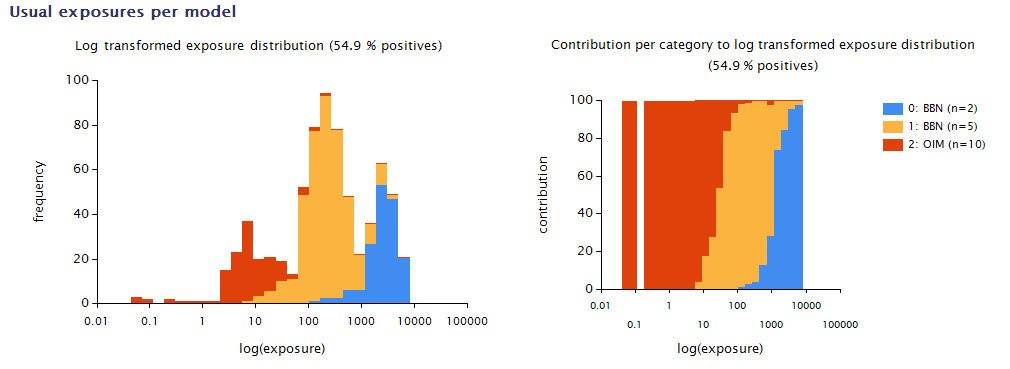
After a split-off selection has been made, the OIM distribution is summarised in terms of the defined grouping (Figure 30), and the usual exposure distribution per split-off food or food group is fitted according to the chosen modelling settings.

Figure 30 OIM usual exposure distribution showing the contributions from the three food groups as constructed in Figure 29.

The Add step

Consumptions of foods may be correlated. In the traditional Add-Then-Model approach the Add step automatically reflects any correlations that are apparent in the consumptions at the individual-day or individual level. In the Model-Then-Add approach the estimated usual exposure distributions for different foods or food groups have to be combined to assess the total usual exposure. Two approaches are available for this:

1. Model-based approach: adds independent samples from the usual exposure distribution per food or food group, ignoring any correlations in consumption;

2. Model-assisted approach: adds the model-assisted, person-specific usual exposure estimates per food or food group, taking correlations in consumptions into account.

See also, episodically consumed foods, model-based, model-assisted.

Before the addition is made, in the model-based approach, model-based estimates of the usual exposure amounts distribution per food or food group are back-transformed values from the normal distribution assumed for transformed amounts per food or food group, and the model-based frequency distribution is sampled to decide if a simulated individual has exposure via the food or food group or not. Model-assisted estimates of the usual exposure distribution are back-transformed values from a shrunken version of the transformed OIM distribution, also done per food or food group, where the shrinkage factor is based on the variance components estimated using the linear mixed model for amounts at the transformed scale (van Klaveren et al. 2012). For individuals with no observed exposure (OIM=0) no model-assisted estimate of usual exposure can be made and a model-based replacement is used.

The model-based approach was investigated in Slob et al. (2010) [Slob et al., 2010] and performed surprisingly well, even if correlations in consumptions of foods were present. The model-assisted approach adds exposures at the individual level, and therefore retains effects of correlations between foods in the usual exposure distribution.

MCRA calculates both the model-based and model-assisted usual intake distributions.

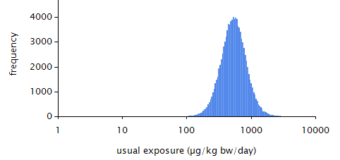
Figure 31 Model-assisted estimated usual exposure distributions (excluding the zero exposures).

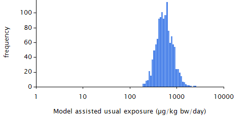
Figure 32 Model-based estimated usual exposure distributions (excluding the zero exposures).